
Last week, Rhett did a post on animating a bouncing ball in VPython. This was mostly making a point about the distinction between real simulation and animation, along the lines of yesterday's post on social construction of videogame reality. But, of course, my immediate reaction was, "That's not how a bouncing ball looks..." This is how a bouncing ball looks:
(As you can see from the watermark, I'm trying out a new video editor...)
This is footage of four different types of balls bouncing on a lab cart in our stockroom, shot in gratuitous slow motion (240 fps) because I'm still playing around with my new camera. These are what I happened to have lying around: a black rubber "happy" ball from a lab set, a hard plastic projectile from a PASCO launcher, a ping-pong ball, and a racquetball. There are some significant differences between them-- the projectile ball stops really quickly, while the ping-pong ball goes on forever-- but they all have one thing in common: the bounce height decreases rapidly as the bouncing goes on.
So, if you want to really animate a bouncing ball, you need to capture that. And, of course, being a great big nerd, I'm far more interested in simulation than animation, so let's think about the physics, here, and how to code it up in VPython.
First and foremost, we need to think about how to handle the bouncing behavior. But, of course, that's pretty easy and obvious, given all the previous futzing around with VPython simulation we've done here: we just treat the ball as a spring. I assigned a fairly arbitrary spring constant to the ball, and put in an if-then statement to apply a spring force if the center of the ball was within a radius of the "floor." Then I fiddled with the spring constant to give reasonable behavior, namely keeping the center of the ball from getting all the way to the floor. That gives you a bouncing behavior that looks just like Rhett's constant acceleration animation:
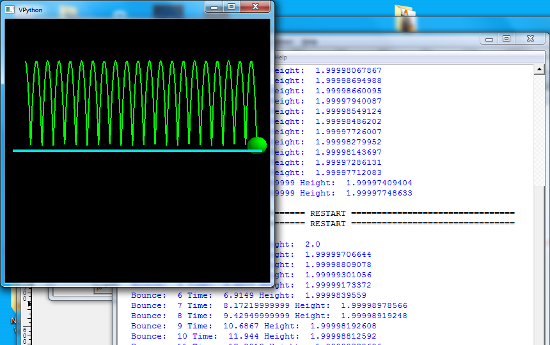 Bouncing ball screenshot with no dissipation.
So, you know, physics works.
Of course, the more interesting question is how to handle the decay of the bounce. To put that in, we need to think about the physics of why it decays. This is easiest to understand in terms of energy: the falling ball has some kinetic energy, and when it hits the table, some of that energy is converted into thermal energy, heating up the ball and the table by a tiny amount. That thermal energy can't be recovered and turned back into energy of motion, so when the ball heads back up, it has less kinetic energy than when it started. That means that when it reaches the peak of its flight, turning all of the kinetic energy into gravitational potential energy, it's not as high as it was on the previous bounce.
So, how to model this? Well, the cheap and easy thing to do would be to just insert a line that automatically decreases the energy when it bounces. But we didn't explicitly calculate the energy of the ball at any point in the simulation above, just the forces that act on in. Besides, we're trying to do physics here.
So, how do you lose energy? Well, introductory Newtonian mechanics tells us that energy is converted to thermal energy through the action of "non-conservative" forces (a term that causes no end of confusion, but we're kind of stuck with it...), which are easiest to understand by considering their opposite.. A "conservative" force is one where the work done as you move between two points is independent of the path you take from one point to the other, and those give you potential energy-- gravity is a good example. As you lift something up, gravity resists your motion, but if you lower it, gravity helps you move it. The total work done by gravity thus depends only on the difference in heights-- if you lift something up above the final position, then lower it back down, gravity resists the motion for part of that, and helps for another part, and those bits cancel each other out.
A non-conservative force, on the other hand, is one where the work done depends on the path that you follow-- a short path means little work, and a longer path requires more work. Friction and air resistance are the classic examples: because friction is always in the direction opposite the direction of motion, it never helps you, and only hurts. A long path means more work against friction, which is why people moving furniture always follow the most direct route they can when sliding stuff across the floor.
So, to lose energy, we want to add a force that is always in the direction opposite the ball's motion. There are two classic, simple mathematical forms for this kind of thing if you're thinking about drag forces on a particle moving in a fluid: For thick fluids, there's a viscous drag force that depends on the velocity, and for thinner ones, there's a drag force that depends on the square of the velocity. Since the VPython simulation tracks velocity directly, as a vector, both of these are easy to implement with an extra line in the if-then statement where I calculate the spring force. Of course, I'm not sure which of these to prefer, so I coded both of them up.
But then, it's not clear why either of those models would apply; they're just convenient and familiar things to add in. The actual dissipation comes about through the motion of the atoms and molecules making up the ball and the table, which aren't necessarily like particles in a fluid. But those are also the very things that give rise to the spring force, so maybe a more appropriate method would be to add a drag force that's a fixed fraction of the spring force (but still always in the direction opposing the motion). That's also pretty easy to do, so I added a third calculation to the loop.
So, what's the end result? Well, here are three traces showing the three different models, for a fairly arbitrary choice of parameters that give 50 bounces before the height of the bounce is less than 5% of the radius of the ball. (This is an unrealistic set of values, but it highlights the difference between the models, and we're just playing at the moment).
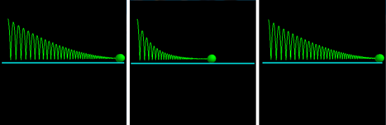 Left: bouncing ball with drag linear in velocity. Middle: bouncing ball with drag quadratic in velocity. Right: bouncing ball with drag a fixed fraction of the spring force.
On the left is the linear-in-velocity drag force, in the middle is the velocity-squared drag force, and on the right is the fraction-of-the-spring-force drag. You can see that there's a big difference between the linear and quadratic models-- the quadratic version dies down much faster, but looks like it sort of levels out and continues at a lower amplitude for a long time. If you can see a difference between the linear and fraction-of-drag models, you've got better eyes than me. In fact, they're nearly identical. Don't believe me? Here are some graphs:
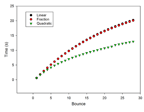 Time of the nth bounce for the simulated ball under the different drag models.
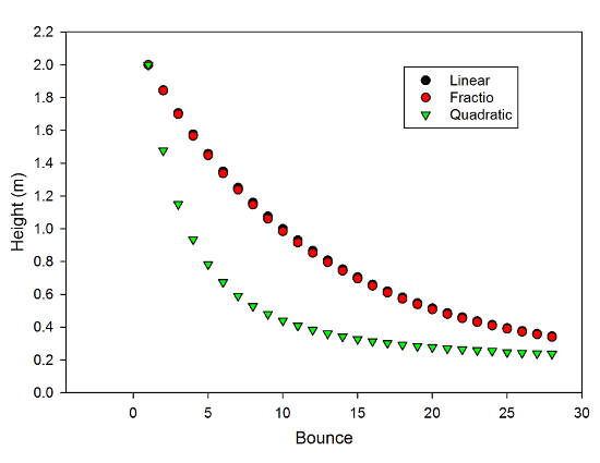 Height of the nth bounce, under three different drag models.
The top graph shows the time of the nth bounce-- defined as the time when VPython noticed that the velocity has changed from down to up-- and the bottom graph shows the height of the nth bounce-- defined as the time when VPython noticed that the velocity has changed from up to down. These are closely related, of course-- the time between bounces is the time to go up to a given height and come back down-- but they're two easy things to measure and graph. And the important thing to notice from these is that there's basically no difference between the linear-drag and fraction-of-spring models. Why is that? I have no idea. If you know, please enlighten me.
So, how do these compare to the real bouncing balls from the video at the top of this post? Well, this is where the gratuitous sow motion kind of bites me in the ass-- analyzing these with Tracker takes frickin' forever because of the high frame rate. I do have numbers for one of the clips, though, but this post is kind of long already, so we'll save that for tomorrow...
In the meantime, if you'd like to play with the simulation yourself, play "find the stupid coding error," or just point and laugh at my rudimentary VPython, the code for this is on Gist. Have fun.
" ...there’s basically no difference between the linear-drag and fraction-of-spring models. Why is that?"
In a very lightly damped harmonic oscillator, which you have here, the velocity is nearly the same as the displacement, shifted by 90 degrees (and with a constant multiplicative factor). So the energy dissipated per bounce for the fraction-of-spring case is like the integral of abs(cos x) over a half cycle, and for the linear drag case it's like the integral of abs(sin x) over a half cycle. And those are the same. Maybe you'll see greater differences if the damping is increased?
Have you addressed why the pingpong ball reverses lateral direction?
I haven't addressed the horizontal reversal of the ping-pong ball. I suspect that's due to air currents of some sort (the open door to the room is to the right of these videos)-- the ping-pong ball is far and away the lightest of the three, and thus the most susceptible to being blown about.
Try it with "identical" Hevea rubber or Superball versus a butyl rubber ball. Restitution matters.
Of course, then there's vibrational modes generated in the ball, the air inside the ball, and the table (the latter should be fairly negligible). These modes may or may not damp (viscoelasticity and other effects) on a reasonable time-scale, affecting restitution. (Surprisingly, I'm in agreement with Uncle Al here.)
This blog post shows direct relation to material I am currently studying in my physics class. The experiment is conducted to show how four different types of balls (rubber, plastic, ping pong and racquetball) bounce upon a surface. They all have significant differences, but one thing remains common to all four. That is, with each bounce, the height the ball reaches continually decreases. The animations show that the kinetic energy is converted into thermal energy, but after hitting a surface, this energy can not be fully recovered back into energy of motion thus decreasing the peak of each following bounce. This is can also be directly related to gravitational pull, velocity and acceleration which are also recently discussed topics in class. The graphs displayed show the bounce vs. time/height correlations, and how all of these factors play a role into each bounce the ball takes. After reading this blog I could take some of the knowledge I have gained in class and apply it to this experiment. It is really neat!
The topic addressed above relates to how the energy of a bouncing ball decreases with time. Several forces act on the ball that decrease its energy with each bounce, several of which have been discussed in class. These include air resistance, friction, gravity, and the opposite but equal force which acts on the ball when it hits the table (Newton's Third Law). The velocity of the ball will decrease with time and distance because of these forces. The reason this ball would not bounce as far as a ping pong ball, for instance, is related to its mass which affects friction. This can be explained by the equation that give kinetic friction: Fk=u(k)mg ; the larger the mass, the higher the friction which in turn will cause the ball to slow down more rapidly. It also relates to what Brittany said above about how the height of the ball decreases with each bounce. The graphs also do a great job of putting the simulation into better terms of understanding for me as we have evaluated similar graphs in class.
When the different balls are dropped and allowed to bounce, they decrease in height after each bounce. In my physics class we talked about a few different topics that relate to this experiment. For example, the constant downward force which is 9.8 m/s^2 is constantly pushing the ball down towards the ground. Also, Newton's Third Law comes into play here. The law states, for every reaction there is an equal and opposite reaction. The opposite reaction in this case is the force that the ground is exerting back on the ball. Finally, this experiment relates to kinetic friction which slows down an objects velocity. Heavier balls such as the first one used in the experiment do not bounce as high because an object with a large mass will have more kinetic friction than an object with a smaller mass, causing it to slow down and not bounce as high.
I really like this topic, because it relates to the current lectures in my physics class. I understand that the main point of this blog was to know that the height of every bounce will decrease as it keeps bouncing. Why? As the ball bounces up it will lose some of its thermal energy, which means it will have less kinetic energy. This also relates to Newton's third law, which says that forces always exist in pairs. This means that in an object there is an equal and opposite reaction. The ball and the ground are the two forces that exist in pairs. For example, the ground will exert the opposite force to the ball. Thank you for the video and graphs that you provided. It made your topic easy to understand.
The most common approach to model the energy loss in this situation is to use a coefficient of restitution (CoR), which here is the ratio of speed of ball before and after collision (assuming the table is stationary). This would predict that the bounce height should decrease in geometric progression with each bounce, and the CoR can be conveniently estimated by sqrt(h/H) where h is first bounce height and H is the initial drop height, and should remain constant with each subsequent bounce.
Of course, this assumes that CoR is independent of impact velocity, which it isn't, and also the bounce height will depend on the rigidity and dimensions of the substrate (try bouncing on stainless steel or plastic to see the difference). Nevertheless, if you analyze your results from your (Hookean) spring model with linear and quadratic damping, you will find that CoR varies with number of bounces in quite an unphysical way. In particular, for quadratic damping, the CoR increases rapidly with each bounce, approaching unity within 20 bounces, which is very unphysical. In plain English, a real ball would not bounce so many times with small amplitude before coming to rest.
To get better predictions, you should use Hertzian elastic theory, which predicts the spring force between sphere and plane close to contact is proportional to deformation ("stretch" in your code) to the power 1.5, not linear. This improves the situation - CoR is now constant to around first 10 bounces, but then starts to increase again. For even better agreement, use a modified form of the linear damping equation with a term involving stretch to the power 0.25.
For a more detailed comparison between linear spring-dashpot model and damped Hertzian oscillator, you can see http://dx.doi.org/10.1209/0295-5075/94/50004